It is widely acknowledged that Data Science involves both modeling and the search for optimal algorithms. However, a well-established reality is that Data Scientists often dedicate a significant portion, around 80%, of their time to Data Collection and Data Preparation, with only 20% of their time allocated to modeling. The features and data quality play a crucial role in enhancing communication with the model and significantly influence its performance. Consequently, investing time in preprocessing is highly worthwhile. It is important to note, however, that superior preprocessing alone does not guarantee the best results; the quality of the data itself is equally vital in achieving optimal outcomes.

Let us dive deep into the steps involved

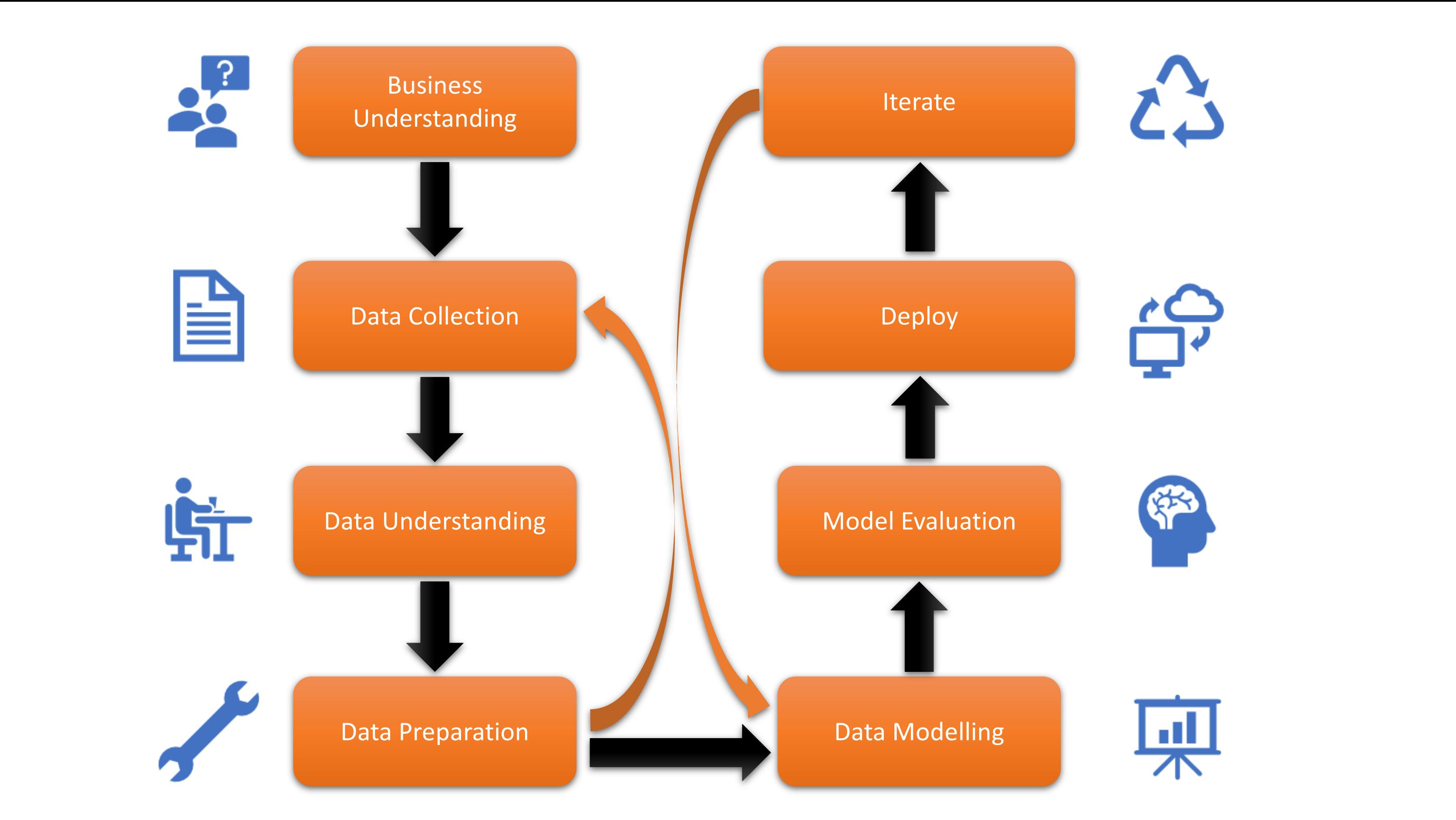
Source: towardsdatascience.com

In this article, the primary focus will be on the data preparation stage. Now that we have understood the importance of data preprocessing in any Data Science project, you might be wondering about the techniques involved and the process. How can it be done? What are the steps involved? Rest assured, I have you covered.

Data Cleaning

The initial step involves Data Cleaning, where we address any inconsistencies or imperfections in the raw data. It is common for raw data to contain issues such as formatting irregularities or data that is not in a suitable format for further analysis. So here is what we need to mainly focus on in the stage of Data Cleaning:

1. Missing values: Instances where data is incomplete or not recorded for certain variables or observations (usually represented as NaN).

2. Inconsistent formats: Data that is not standardized or follows different conventions across variables or observations. Eg:

   a. Consider age: Representing 21 as 21+ or in any other way is invalid.

   b. Categorical variables are represented differently across the dataset, such as using abbreviations, full names, or numerical codes inconsistently.

3. Incorrect data types: Variables assigned with incorrect data types, such as numeric data stored as text or vice versa. Eg:

   a. If the "age" feature is expected to be numerical but is erroneously identified as an 'object' data type, it is crucial to investigate why this misclassification occurs. By examining the underlying reasons for the incorrect data type, such as missing values or non-numeric characters, we can take appropriate measures to resolve these issues. Applying the necessary data cleaning steps and utilizing the astype function can help ensure that the "age" feature is properly converted to the desired 'int' data type.

4. Duplicate records: Instances where identical or nearly identical data entries exist within the dataset, leading to redundancy. Duplicates induce bias in the model hence we need to deal appropriately.

5. Data entry errors: Typos, misspellings, or incorrect values entered during data collection or input.

6. Outliers: Data points that deviate significantly from the expected or typical values, which may be due to measurement errors or anomalies.

Data Wrangling / Data Transformations

It is all about transforming the data from one format to the other, crucial steps involved in Data transformations are

1. Discretization / Binning / Bucketizing: The process of discretization aids in the efficient analysis of data, particularly when dealing with continuous variables (but not restricted to) that pose challenges in their raw form.

   Let's consider an example: if we have 100 distinct values for the "age" variable, it can be simplified by grouping the data into age categories such as child, teen, adult, etc. This allows for easier interpretation and analysis of the data. Discretization involves dividing a continuous variable into meaningful intervals or categories, providing a more manageable representation for further analysis and interpretation.

   Note: Discretization is not a mandatory step that must be performed before commencing modeling; rather, it is an optional technique that offers a convenient approach to data analysis.

   • Are there any advantages of doing this apart from helping in analysis? Certainly!

     • Prevents overfitting, reducing the model complexity

     • Increase the robustness of the model to anomalies

2. Encoding: While most machine learning algorithms typically cannot directly handle categorical data, it is common to encounter categorical variables in our datasets. However, this does not mean that we cannot include categorical variables in our analysis. To enable the utilization of categorical variables, they must be encoded using appropriate techniques such as Label Encoding or One Hot Encoding, depending on the nature of the categorical variable.

   • Label Encoding involves assigning a unique numerical label to each category within a variable, effectively converting it into a numerical representation. This method is suitable for variables with an inherent ordinal relationship among the categories.

   • One Hot Encoding transforms each category within a variable into a separate binary column. Each column represents a specific category, and a value of 1 is assigned if the observation belongs to that category, while 0 is assigned for all other categories. This approach is useful for variables without any inherent ordinal relationship, as it avoids imposing any artificial order among the categories.

     • The disadvantage with the one hot encoding is that there will be a significant increase in the size of the dataset especially when a variable contains a huge number of unique values

Note: Encoding is a mandatory step that must be performed (for most of the algorithms)

1. Scaling: Scaling is a valuable technique that contributes to improved results in machine learning. It is particularly useful for algorithms that utilize distance-based concepts. While not every algorithm is sensitive to scaling, there are certain cases where scaling is mandatory to achieve efficient and accurate outcomes. Algorithms such as Decision Trees and Random Forests are inherently robust to scaling. They can handle features with varying scales without compromising their performance. However, other algorithms like K-Nearest Neighbors (KNN), Support Vector Machines (SVM), Principal Component Analysis (PCA), and Regularization-based models require scaling for optimal results.

   Scaling is crucial for KNN as it relies heavily on distance calculations between data points. If the features are not scaled, those with larger scales may dominate the distance calculations, leading to biased results. Similarly, SVM and PCA benefit from scaling as it ensures that all features contribute equally and accurately to the models' decision-making process.

   For Regularization-based models, scaling prevents features with larger scales from disproportionately influencing the regularization term, leading to more balanced and reliable results, hence scaling is needed to bring all the values to the same scale.

   • There are different techniques of scaling:

     • MinMaxScaling: Minimum and Maximum values are considered (Normalization - range [0,1])

     • Standard Scaling: Mean and standard deviation values are considered (Standardization - range [-4,4])

Note: This is not mandatory but produces better results on sensitive to scaling algorithms

1. Transformation: Transformation is a valuable technique that enhances the model's performance. Many machine learning algorithms are based on the assumption that the data follows a Normal or Gaussian distribution, where the data is roughly distributed under the bell curve. However, not all variables in our dataset necessarily adhere to this normal distribution. Some variables may exhibit left or right skewness.

   To address this issue, transforming skewed variables into a Gaussian distribution can be an effective approach. By applying appropriate transformations, such as logarithmic, square root, or Box-Cox transformations, we can reshape the variable's distribution and bring it closer to the desired Gaussian distribution. This helps to align the data with the assumptions of the machine learning algorithms, thereby improving their performance and yielding more reliable results.

Summary

The techniques discussed in this article contribute to an enhanced data preprocessing process, leading to improved and generalized results. Understanding the applications, advantages, and disadvantages of these techniques ensures a seamless and effective implementation. By incorporating these insights into your data preprocessing workflow, you can optimize the quality and reliability of your analyses and model outcomes.

#important imports
import numpy as np
import pandas as pd
from sklearn.impute import SimpleImputer, KNNImputer
from sklearn.preprocessing import LabelEncoder, OneHotEncoder, MinMaxScaler, StandardScaler
from sklearn.preprocessing import PowerTransformer
from scipy.stats import boxcox

Thanks for reading! KnowledgeIsFun